Thoughts on FOSS4G NA 2016

This year’s Free and Open Source for Geospatial (FOSS4G) North America event was held in Raleigh, NC between May 2-5, 2016. Attendance increased by 150+ over last year, bringing the total to over 550 registrations. While typically a developer conference with technical software presentations, recent years has seen an increase in participation (both attendance and presentations) from the user community. This year continued that trend, and the agenda included a wide array of topics. In addition to good facilities and well run logistics, the program committee did an excellent job curating the presentations; nearly all of the sessions I attended were appropriate content and well delivered, a feat for any conference. A full list of the attended sessions I attended is in the table at the end of the post.

Below are some of my takeaways from the conference, categorized into three general themes: Tools, Data, and Visualization.

Tools

It is clear that open source software continues to mature, and when combined with new deployment technologies like Docker containers and cloud, it is a fundamentally different world than a few years ago. This is clearly not a ground shaking statement, but the speed by which anyone can go from zero to a cloud-deployed, scalable geographic computing infrastructure is amazing.

Machine Learning is everywhere. Granted I haven’t used ML approaches in a few years, but my concern is that simpler approaches of statistical modeling are being overlooked just to use the big, new shiny thing. The underlying assumption with ML is that all problems are solved best through inductive methods, which potentially discounts the wisdom of domain expertise. ML is obviously very powerful when lots of data is available and should be part of the modelling toolkit, but it’s not a magic bullet and mis-applications are going to become more common. Using TensorFlow or the other new algorithms doesn’t fundamentally change the need to understand how statistics and modeling works, and modelers need to be aware of the full range of statistical tools.

On the Natural Language Processing (NLP) and geocoding side, GeoParser could be key bridge between the document open data and geospatial open data communities. Combining tools like Apache Tika, Stanford NLP, and Gazetteer lookup means there is a single toolkit with the potential to geocode any document. Clearly geocoding results here are limited in success to the quality of the gazetteer, but the processing pipeline is interesting.

The Geo Big Data processing tools continue to mature and are even starting to converge on the use of underlying libraries and database. This collection of tools includes GeoWave, GeoTrellis, GeoMesa, GeoJinni. Personally I’m interested in the use of GeoTrellis for high-performance raster modeling.

Sensors are expanding everywhere: agriculture best example of persistent, integrated data collection across sensors (imagery, lidar, IoT) and application into “smart” devices (self-driving farm equipment and custom planting / harvesting strategies). OpenSensorHub can be used to integrate various feeds, thinking of applications with automated hydromet, weather, and seismic stations, as well as other crowd reported data feeds.

Data

Vector tiles expand market share: nascent analytical capability, new version 2.0 specification, true 3D in the tile (when comes 4D), added to GeoServer

Remote Sensing is big: Cubesats, Drones, Imagery, Point Clouds all continue to grow and expand into all market verticals (farming, logistics, business analysis leading the way)

Remote Sensing is still hard: massive imagery catalogs only further expose fundamental remote sensing issues on analysis (orthorectification and image-to-image registration, atmospheric effects on spectral reflectance); drones and kites driving new photogrammetric toolkits; the cool kids are yet to fully catch on to these challenges.

OSM ecosystem continues to deepen and expand: Portable OpenStreetMap, or POSM, is a nice tool for enabling disconnected editing in austere environments. The upgraded HOT Export Tool is a key part of exporting the initial datasets used for the process. The critical question is how to get data back into OSM. Currently all edits are manually reviewed, using an interesting queuing mechanism that maintains individual changesets, and then uploaded using an import account. The question is how will the method scale when remote mapping is occurring at the same time as field mapping, the potential disconnect between edit histories of the disconnected branch can and will be an issue.

Visualization

Vector tiles is driving more client side rendering. Mapbox obviously leading the way here, but Boundless now supporting vector tiles in GeoServer and OpenLayers.

Seamless 2D/3D visualization: Cesium is everywhere, TerriaJS interesting library to add better visualization on top of spatial data catalogs; USGS/NASA GIBS adding atmospheric data slices into dense imagery catalogs. When do we get 4D tiles and/or tiles with multiple versions of the same dataset?

Imagery is driving client side visualization and nascent imagery exploitation tools in the browser

Convergence of ground based and aerial based views: “painted” 3D models from photogrammetric extraction combined with Mapillary type imagery; farm management using ground and aerial lidar clouds.

Sessions

Each of the links below go to the FOSS4G session page, many of which have links to the slidedecks and in the coming weeks will have the video recording of the presentation.

The US National Spatial Data Infrastructure: Where do we go from here?
Precision Agriculture and Open Spatial Technologies
Mapping the Planet from Outer Space
Climbing the data mountain: Scaling and optimizing the delivery of vector tiles
Mapbox Vector Tile Specification 2.0
Open Source Photogrammetry with OpenDroneMap
Image Mosaics & Automation
Memex-GeoParser
MARPLOT: Building a Desktop GIS for Emergency Response from FOSS Components
In-browser, scale-independent geo data analysis using vector tiles
Portable OSM – OSM in the Disconnected Wilds
New features in WhirlyGlobe-Maply Version 2.4 and Beyond
3D Tiles: Beyond 2D Tiling
OpenSensorHub for SensorWebs and IoT
Geo(Mesa/Wave/Trellis/Jinni): Processing Geospatial Data at Scale @locationtech
GeoMesa, GeoBench, and SFCurve: Measuring and improving BigGeo performance
Developing a Geospatially Explicit U.S. Synthetic Population Using Open Source Tools
Pixel Gymnastics Using OpenLayers and Planet Labs Data
Machine Learning on Geospatial Datasets for Segmentation, Prediction and Modeling
Automated High Resolution Land Cover Generation from WorldView Multispectral Imagery
Point cloud web services with Greyhound, Entwine, and PDAL
Spatial Data Processing with Docker
Vector Tiles with GeoServer and OpenLayers

In the next post, I’ll cover the workshop section of the conference.

Print Friendly, PDF & Email

World Country Polygon Datasets

The Humanitarian Information Unit (HIU) has released several new datasets that leverage the Office of the Geographer‘s work on mapping International Boundaries. The Large Scale International Boundaries (LSIB) dataset, maintained by the Geographic Information Unit (GIU), is a vector line file that is believed to be the most accurate worldwide (non-Europe, non-US) international boundary vector line file available. The lines reflect U.S. government (USG) policy and thus not necessarily de facto control (cited from metadata attached to files). In September 2011, the HIU first released the boundaries publicly for download. Working with colleagues at DevelopmentSeed after that release, they made some substantial improvements to the underlying data structure that helped lead to this work.

The LSIB dataset is designed for cartographic representation and map production. However, this poses a problem for GIS analysis, because the dataset is only composed of vector lines of terrestrial boundaries between countries. This means they do not contain coastlines, and could not be converted into polygons for GIS analysis. To address this issue, the HIU combined the LSIB dataset with the World Vector Shorelines (1:250,000) dataset. The combination of these two datasets is one of the highest resolution country polygon datasets available. Additionally, the LSIB-WVS polygon file is believed to be the most accurate available dataset for determining island sovereignty. It corrects the numerous island sovereignty mistakes in the original WVS data (cited from metadata attached to files).

Two other modifications were made to the datasets. First, the large cartographic scale of the data also introduces a problem in that the data are too detailed for global scale mapping. Therefore, the HIU also created “generalized” versions of the original LSIB-WVS polygons that are suitable for smaller scale mapping. Second, in order to facilitate the ability to “join” data to the polygons in a GIS, several attributes were added to the database, including Country Name and several ISO 3166-1 Country Codes (ISO Alpha 2, ISO Alpha 3, and ISO Number). After a year of work, the data have been released into the public domain.

All datasets can be downloaded from the HIU Data page or the links below:

LSIB – WVS Country Polygons

High Resolution LSIB-WVS Country Polygons (Americas) :: https://hiu.state.gov/data/Americas_LSIBPolygons_2013March08_HIU_USDoS.zip

High Resolution LSIB-WVS Country Polygons (Africa/Eurasia) :: https://hiu.state.gov/data/EurasiaAfrica_LSIBPolygons_2013March08_HIU_USDoS.zip

Simplified Versions

Simplified Global World Vector Shorelines :: https://hiu.state.gov/data/Global_SimplifiedShoreline_2013March08_HIU_USDoS.zip

Simplified Global Country Polygons :: https://hiu.state.gov/data/Global_LSIBSimplifiedPolygons_2013March08_HIU_USDoS.zip

LSIB Lines

Large Scale International Boundaries (LSIB), AFRICA and the AMERICAS :: https://hiu.state.gov/data/AFRICAandAMERICAS_LSIB4b_2012Sep04_USDoS_HIU.zip

Large Scale International Boundaries (LSIB), EURASIA :: https://hiu.state.gov/data/EURASIA_LSIB4b_2012Sep04_USDoS_HIU.zip

Cartographic Guidance

Note, both the polygon and line datasets are useful for cartographic representation. This is due to the variety of different boundary classifications that are in the LSIB. Below is a subset from the metadata attached to the datasets that describes USG cartographic representation of the boundary lines.

From the LSIB lines metadata:
The “Label” attribute field provides a name for any line requiring non-standard depiction, such as “1949 Armistice Line” or “DMZ”

The “Rank” attribute categorizes lines into one of three categories:
a) A rank of “1” (includes most of the 320 international boundaries) for those which the USG considers “full international boundaries.”
b) A rank of “3” for other lines of international separation. Most are considered by the US government to be in dispute.
c) A rank of “7” for other lines of separation such as DMZ’s, No-Mans Land (Israel), UNDOF zone lines (Golan Hts.), Sudan’s Abyei, and for the US Naval Base Guantanamo Bay on Cuba.

Any line with a rank of “3” or “7” is to be dotted or dashed differently and in a manner visually subordinate to the normal rank “1” lines.

Additional information about how the LSIB dataset is produced, and the processes that went into the production of the new datasets are included in the metadata.

And for more information about the Office of the Geographer, see the article from State Magazine below:

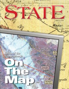
State Magazine (March 2009) Office of the Geographer
Article about the Office of the Geographer from State Magazine in March 2009
Print Friendly, PDF & Email

Modifying the KARS GeoNetwork metadata catalog

We recently had an inquiry at the Kansas Applied Remote Sensing Program (KARS) about modifications we made to our GeoNetwork instance. Specifically, the question was about setting the Intermap window to open in the large format on load, and setting the map extent.

We run the Windows version of GeoNetwork and have used these modifications for Versions 2.2, 2.4.2, and 2.4.3.

First, to call the Intermap function we modified the following files:
\geonetwork\web\geonetwork\xsl\main.xsl
\geonetwork\web\geonetwork\xsl\main-page.xsl
\geonetwork\web\geonetwork\geonetwork.css

1) main.xsl – @ line 18 added ‘openIntermap’ function call to the onLoad event


<body onload="init(), openIntermap()">

2) main-page.xsl – @ line 281, “fillMeWithIntermap”, add ‘width: 700px;’

<tr id="intermaprow"  width="100%" height="0">
  <xsl:comment>COLLAPSABLE MAP</xsl:comment>
    <td>
      <strong><div id="fillMeWithIntermap" style="display: none; width: 700px;"></strong>
      <!--  This DIV will be filled dynamically with intermap contents -->
      </div>
    </td>
</tr>

Note that this modification did require some additional CSS modifications, specifically the Z-Index of the map elements had to be re-ordered so they would be drawn last.

Second, modifying the properties that Intermap used at load were modified in the file:
\geonetwork\web\intermap\scripts\im_bigmap.js

3) In row 19 and 20, change the initial width and height of window from w=368 h=276 to w=450 h=300.

 // these are the values of initial width and height. 
var im_bm_wsize0 = 450;
var im_bm_hsize0 = 300;

4) Inserted a line (line 19) to define the map extent (zoom) of the Intermap big map window to North America.

 Line 19: im_bm.setBBox(51.56155, -66.07543, 21.629387, -125.93976)
Line 20 for comments: // view of the United States (minx="-125.93976" miny="21.629387" maxx="-66.07543" maxy="51.56155") 

5) Modified the default scale zoom parameters for the intermap window on load to include 1:24,000.
File: \geonetwork\web\intermap\xsl\index-embedded.xsl

At line 141, an option for the value “24000” was added


<select name="im_setscale" id="im_setscale" onchange="javascript:im_bm_setScale();">
<option id="im_currentscale" value=""><xsl:value-of select="/root/gui/strings/setScale</option>                    
    <option value="50000000">1:50.000.000</option>
    <option value="10000000">1:10.000.000</option>
    <option value="5000000">1:5.000.000</option>
    <option value="1000000">1:1.000.000</option>
    <option value="500000">1:500.000</option>
    <option value="100000">1:100.000</option>
    <option value="50000">1:50.000</option>
    <option value="24000">1:24.000</option>
    <option value="10000">1:10.000</option>
    <option value="5000">1:5.000</option>
    <option value="1000">1:1.000</option>                    
</select>

Additional modifications can be found in the following document KBS_GeoNetwork_Modifications. Any comments or additional suggestions for modifications are welcome.

Print Friendly, PDF & Email